Lesson 7 of 9
Module 3 · Figures that tell the truth
Heatmaps, volcano plots and MA plots summarise thousands of genes in one picture. Each has a few choices that decide whether it informs or misleads.
Clustered heatmap
Scale each gene (row) to z-scores, so colour shows each gene relative to its own average; otherwise a few highly expressed genes take all the colour. Clustering then groups similar genes and samples.
Here is why scaling matters. Suppose gene A has values around 10,000 and gene B values around 50. On one shared colour scale, gene A is dark red in every sample and gene B is pale in every sample, so neither shows any difference between control and treated. After z-scoring, each gene's own mean becomes 0 and its own standard deviation becomes 1, so a sample coloured red is above that gene's average and one coloured blue is below it, whatever the gene's absolute level.
Clustering (here, hierarchical clustering) repeatedly joins the two most similar rows, or columns, into a group, and draws the joins as a tree called a dendrogram along the edge of the heatmap. Rows are then reordered so similar genes sit next to each other, which is what turns scattered colours into visible blocks.
The matrix z comes from Colour that works for everyone, where each gene in expression_example.csv was z-scored with t(scale(t(...))) and drawn in a blue–white–red palette with clustering switched off. This lesson keeps the same colours and lets pheatmap reorder the rows and columns. The direction of scaling matters. scale() works on columns, which is why the matrix is transposed before and after; scaling the samples instead of the genes would leave the highly expressed genes dominating the colour, the very problem z-scoring by gene is meant to solve.
ann <- data.frame(group = rep(c("control", "treated"), each = 4), row.names = colnames(z))
pheatmap(z, annotation_col = ann,
         annotation_colors = list(group = c(control = "#0072B2", treated = "#E69F00")),
         color = colorRampPalette(c("#2166AC", "white", "#B2182B"))(100),
         breaks = seq(-2.5, 2.5, length.out = 101))
What this does
- The first line builds a small table,
ann, describing the samples.rep(c("control", "treated"), each = 4)gives "control" four times and then "treated" four times, one label for each of the 8 samples.row.names = colnames(z)names each row after a column ofz, which is how pheatmap knows which label belongs to which sample. pheatmap(z, annotation_col = ann, ...)draws the z-score matrix from Colour that works for everyone and adds a coloured bar above the columns showing each sample's group.annotation_colorssets the colours of that bar: blue for control and orange for treated, from the Okabe–Ito palette.colorandbreakswork as in Colour that works for everyone: 100 colours from blue through white to red, with 101 cut points spread evenly from −2.5 to 2.5, so white falls exactly at 0.- Rows and columns are clustered, because pheatmap clusters both by default; Colour that works for everyone switched this off to keep the original order.

Reading the heatmap
Start with the column dendrogram and the group bar: if the samples split cleanly into control and treated, treatment is the main source of difference between them. Then read the blocks of rows. A block red in treated and blue in control holds genes that rise with treatment; the opposite pattern holds genes that fall. Rows with no clear pattern are genes that did not respond. A common mistake is to treat the clusters as proof: clustering always produces a tree, even from random numbers, so the blocks are a picture to check against the statistics, not a test.
Remember also what the z-scores remove. Every row now has the same average and the same spread, so the heatmap cannot tell you whether a gene is expressed at 50 counts or at 10,000, nor how large its change is in absolute terms. A gene with a small but very consistent change can look as vivid as one that changes tenfold. Read the heatmap for patterns across samples, and go back to the results table for effect sizes.
Go deeper: what distance the clustering uses
pheatmap measures how alike two rows are with Euclidean distance by default: the straight-line distance between their values. On raw values that groups genes by level, so two highly expressed genes look similar even if one rises and the other falls. On z-scores it behaves differently. For two z-scored genes measured in n samples, the squared Euclidean distance equals 2(n − 1)(1 − r), where r is their correlation. So on z-scored rows, Euclidean distance ranks gene pairs exactly as correlation does, and genes with the same up-and-down pattern cluster together whatever their level.
To cluster unscaled values by pattern, ask for it directly: pheatmap(mat, clustering_distance_rows = "correlation"). The linkage rule, which sets the distance between groups once they form, also matters; pheatmap uses clustering_method = "complete" by default, and changing it can reorder the tree noticeably.
Volcano and MA plots
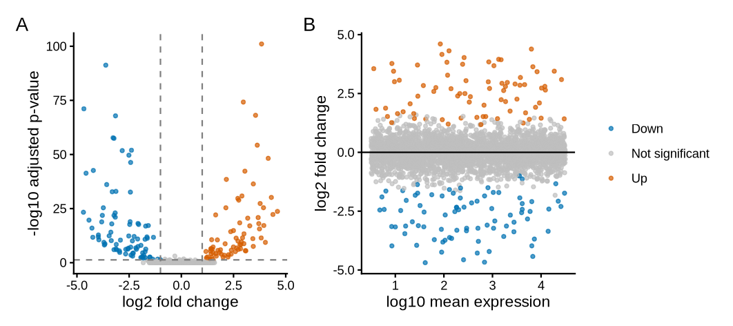
A volcano plot shows effect size against evidence. An MA plot shows effect size against how highly a gene is expressed, which reveals whether low-count genes are driving the results.
The terms come from the columns of a differential expression table, which Module 4 produces for real data. The log2 fold change is the effect size: how much a gene changes between groups, on a log2 scale where +1 is a doubling and −1 a halving. The adjusted p-value (padj) is the evidence, corrected for testing thousands of genes at once. baseMean is the gene's average normalised count, its expression level. The volcano plot takes its name from its shape: most genes form a low mound around zero change, and the strongly changed genes spray up and outwards on both sides. The names M and A come from older microarray work: M is the log ratio and A the average level.
Two choices in the volcano plot need explaining. The y-axis uses the adjusted p-value rather than the raw one because, with thousands of genes, about 5% of the genes with no real change would fall below p = 0.05 by chance alone; Multiple testing and power showed how the Benjamini–Hochberg adjustment keeps these false hits in check. The plot also applies two thresholds at once, because each guards against a different mistake: a large fold change with weak evidence may be noise, and a tiny fold change with strong evidence may be real but of little biological interest.
de <- read.csv("de_results_example.csv")
de$status <- "Not significant"
de$status[de$padj < 0.05 & de$log2FoldChange >  1] <- "Up"
de$status[de$padj < 0.05 & de$log2FoldChange < -1] <- "Down"
table(de$status)

cols <- c(Up = "#D55E00", Down = "#0072B2", "Not significant" = "grey75")
pv <- ggplot(de, aes(log2FoldChange, -log10(padj), colour = status)) +
  geom_point(size = 1, alpha = 0.7) +
  geom_vline(xintercept = c(-1, 1), linetype = "dashed", colour = "grey50") +
  geom_hline(yintercept = -log10(0.05), linetype = "dashed", colour = "grey50") +
  scale_colour_manual(values = cols) +
  labs(x = "log2 fold change", y = "-log10 adjusted p-value", colour = NULL) +
  theme_classic(base_size = 11)
ma <- ggplot(de, aes(log10(baseMean), log2FoldChange, colour = status)) +
  geom_point(size = 1, alpha = 0.7) +
  geom_hline(yintercept = 0) +
  scale_colour_manual(values = cols) +
  labs(x = "log10 mean expression", y = "log2 fold change", colour = NULL) +
  theme_classic(base_size = 11)
pv + ma + plot_layout(guides = "collect") + plot_annotation(tag_levels = "A")
What this does, block by block
- Labelling. After reading the results file, every gene starts as "Not significant". The next two lines overwrite that label for genes that pass both tests:
padj < 0.05and a log2 fold change above 1 (labelled "Up") or below −1 ("Down"). The&means "and".table(de$status)counts how many genes carry each label. - Colours.
colsis a named vector: vermilion-orange for up, blue for down, light grey for the rest, so the eye goes to the significant genes first. - Volcano,
pv. The x-axis is the log2 fold change and the y-axis is-log10(padj). Taking −log10 turns small p-values into large numbers, so the strongest evidence sits at the top.geom_vline()draws dashed lines at −1 and 1, andgeom_hline()a dashed line at the height that corresponds to padj = 0.05. - MA plot,
ma. The x-axis islog10(baseMean), the expression level on a log scale, and the y-axis the log2 fold change.geom_hline(yintercept = 0)marks "no change". - Assembly.
plot_layout(guides = "collect")merges the two identical legends into one, andplot_annotation(tag_levels = "A")labels the panels A and B.
Reading the output
table() prints each label with its count beneath it, in alphabetical order: 83 genes down, 2,841 not significant and 76 up. The three counts add up to 83 + 2,841 + 76 = 3,000, the number of genes in the file, which is a quick check that every gene received exactly one label.
The number of significant genes is not a fixed property of the biology. With more samples per group, smaller changes reach significance and the count grows; with a stricter fold-change cut-off it shrinks. Report the thresholds alongside the counts, as the worked example below does, so that a reader can compare your 159 genes with someone else's.
Worked example · what the thresholds mean
horizontal line at −log10(0.05) = 1.3 → padj = 0.05
significant: 76 up + 83 down = 159 of 3,000 genes (5.3%)
Step by step. A log2 fold change of 1 means a ratio of 21 = 2, and −1 means 2−1 = ½. For the horizontal line, log10(0.05) = −1.30, so −log10(0.05) = 1.30. Reading the axis the other way, a gene at height 2 has padj = 10−2 = 0.01, and one at height 3 has padj = 10−3 = 0.001. For the share: 159 ÷ 3,000 = 0.053, or 5.3%.
What the answer means. Each step up the y-axis is ten times stronger evidence. The fold-change cut-off of ±1 is a convention that keeps only changes large enough to be biologically interesting; it is a choice, and you should state it in your methods.
What the MA plot adds
In panel B, the significant genes are spread across all expression levels. That is reassuring. If the coloured points sat only at the far left, among genes with very few reads, the "changes" could be driven by noise: a gene going from 2 reads to 8 is a fourfold change on paper, but such small counts vary a lot by chance. The MA plot is where you would spot that problem.
In real RNA-seq data the MA plot usually has a characteristic shape: the cloud of grey points is wider at the left, among weakly expressed genes, and narrows towards the right. Low counts carry more chance variation, so their fold changes scatter more. Module 4 meets this with real data, where DESeq2 can shrink the noisy fold changes of low-count genes towards zero before they are plotted. Both panels also follow Honest axes and scales: fold changes are on a log2 axis, so doubling and halving sit at equal distances from 0, and expression is on a log10 axis, because counts span several orders of magnitude.
MA plots come from two-colour microarray analysis; an early, widely cited use is Dudoit, Yang, Callow & Speed 2002, "Statistical methods for identifying differentially expressed genes in replicated cDNA microarray experiments" (Statistica Sinica). The packages used here are pheatmap, by Raivo Kolde, and ggrepel, by Kamil Slowikowski, both on CRAN; cite them with citation("pheatmap") and citation("ggrepel") and give their versions. The cut-offs of padj < 0.05 and a log2 fold change of ±1 are conventions, not standards from any paper. State both in the legend and the methods, because a different choice changes which genes are coloured.
Key point
Label only the genes you discuss, with lines to their points if crowded (the ggrepel package does this). Thirty overlapping labels help nobody.
The same rule applies to the heatmap. With 30 genes, row names are readable; with 2,000 genes they become a grey smear. In that case, hide the row names and say in the legend how many genes are shown and how they were chosen, for example "the 50 genes with the smallest adjusted p-values".
Further reading · Module 3Weissgerber et al. 2015: why bar charts hide the data, with examples. · All reading for this course
Check your understanding
1. Why z-score genes before a heatmap?
2. What does an MA plot add to a volcano plot?
3. On a volcano plot, a gene sits at y = 3. What is its adjusted p-value?
Up next
Lesson 8
Publication-ready export